A Journey to Ito Calculus (not yet to be published)

Random walk

• Consider independent random variables $\{X(n)\}_{n\geq 0}$ with $X(0)=0$ such that $P(X(n)=1)=P(X(n)=-1)=\dfrac{1}{2}$ for $n\geq 1$. Then
  \begin{align} \mathbb{E}[X(n)]&=1\cdot \dfrac{1}{2}+(-1)\cdot \dfrac{1}{2}=0, \\ \mathbb{V}[X(n)]&=\mathbb{E}[X(n)^2]-\mathbb{E}[X(n)]^2=1^2\cdot \dfrac{1}{2}+(-1)^2\cdot \dfrac{1}{2}-0=1 \end{align}
• Let $S(n):=\sum_{j=1}^n{X_j}$. $S(n)$ is called random walk. Also, we see that
  \begin{align} \mathbb{E}[S(n)]&=\sum_{j=1}^n\mathbb{E}[X_j]=0, \\ \mathbb{V}[S(n)]&=\sum_{j=1}^n\mathbb{V}[X_j]+2\sum_{1 \leq i < j \leq n} \underbrace{\text{Cov}(X_i, X_j)}_{=0}\\ &=\sum_{j=1}^n\mathbb{V}[X_j]\\ &=n \end{align}
• From CLT, $\dfrac{S(n)}{\sqrt{n}}\xrightarrow{d} \mathbfcal{N}(0,1)$ as $n\to\infty$.
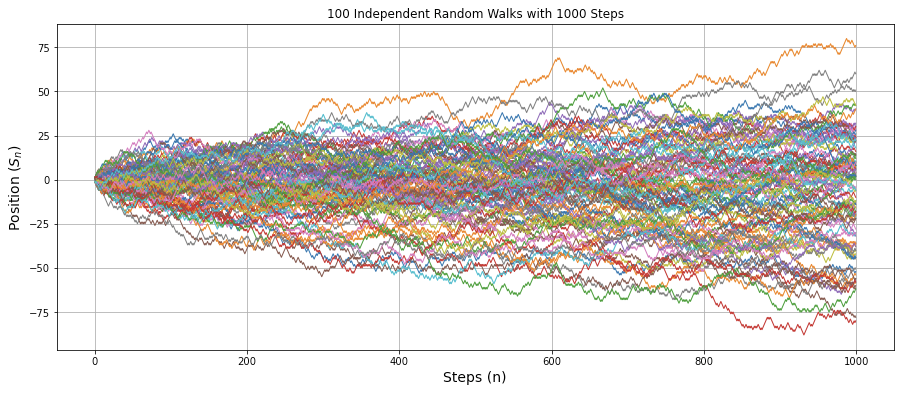  Simulation of 100 independent random walks with 1000 steps

Brownian motion

• Let's rescale the random walk.
• Let $h=\dfrac{1}{N}$ from some $N\in\mathbb{N}$. Consider $\{X_h(n)\}_{n\geq 1}$ such that $X_{h}(n):=\sqrt{h}X(n)$.
• For $t=nh=\dfrac{n}{N}$, let $S_{h}(t):=\sum_{j=1}^n{X_{h}(j)}=\sqrt{h}S(n)$. So
  $S_{h}(t)=\dfrac{1}{\sqrt{N}}S({tN})=\sqrt{t}\cdot\underbrace{\dfrac{1}{\sqrt{tN}}S({tN})}_{\xrightarrow{d} N(0,1)}\xrightarrow{d} \mathbfcal{N}(0,t)$ as $N\to\infty$.
  Simulation of 1000 independent rescaled random walks whose distribution converges to normal distribution as $N\to\infty$. Here we take $N=1000$.
• Formally speaking, a Brownian motion $\{B(t)\}_{t\geq 0}$ is the limit of $\{S_h(t)\}_{t\geq 0}$ as $N\to\infty$.

Construction of Brownian motion (Lévy–Ciesielski construction)

Step 1

• Consider the family $\{h_k(t)\}_{k=0}^{\infty}$ of Haar functions defined for $ 0\leq t\leq 1$ as follows:
  $h_0(t):=1,\quad 0\leq t\leq 1$
  $$ h_1(t):= \begin{cases} 1, & \quad 0\leq t\leq \frac{1}{2}\\ -1, & \quad \frac{1}{2}< x\leq 1\\ \end{cases} $$
  and for $2^n\leq k<2^{n+1},n=1,2,\cdots,$ we set
  $$ h_k(t):= \begin{cases} 2^{n/2}, & \quad \frac{k-2^n}{2^n}\leq t\leq\frac{k-2^n+1/2}{2^n}\\ -2^{n/2}, & \quad \frac{k-2^n+1/2}{2^n}< t\leq \frac{k-2^n+1}{2^n}\\ 0, & \quad \text{otherwise} \end{cases} $$
• The functions $\{h_k(t)\}_{k=0}^{\infty}$ form a complete, orthonormal basis of $L^2(0,1)$.

Step 2

For $k=1,2,\cdots$, define
$$ s_k(t):=\int_0^th_k(s)ds\quad (0\leq t\leq 1) $$
called the k-th Schauder function.

Step 3

Let $\{A_k\}_{k=0}^{\infty}$ be a sequence of independent, $\mathbfcal{N}(0,1)$ random variables defined on some probability space. Then
$$ \textcolor{blue}{B(t,\omega):=\sum_{k=0}^{\infty}A_k(\omega)s_k(t)}\quad (0\leq t\leq 1) $$
converges uniformly in $t$ for a.e. $\omega$. Furthermore,

1. $\{B(t)\}_{t\geq 0}$ is a Brownian motion for $ 0\leq t\leq 1$, and
2. $t\mapsto B(t,\omega)$ is continuous for a.e. $\omega$.

Hence we have constructed Brownian motion on $ 0\leq t\leq 1$.

Step 4

• Reindex $\{A_k\}_{k=0}^{\infty}$ to obtain countably many families of countably many $\mathbfcal{N}(0,1)$ random variables.
• For each family $\{A_k^{(n)}\}_{k=0}^{\infty} ,(n=1,2,\cdots)$, we can build independent Brownian motions $B^{(n)}(t):=\sum_{k=0}^{\infty}A_k^{(n)}s_k(t)$.
• Now paste each Brownian motion inductively as
  \begin{align} B(t)&:=B^{(1)}(t), \quad 0\leq t\leq 1\\ B(t)&:=B(1)+B^{(2)}(t-1), \quad 1\leq t\leq 2\\ B(t)&:=B(2)+B^{(3)}(t-2), \quad 2\leq t\leq 3\\ &\vdots\\ B(t)&:=B(n-1)+B^{(n)}(t-(n-1)), \quad n-1\leq t\leq n \end{align}
  Then $B(t)$ is a Brownian motion for all $t\geq 0$.