exp(共変微分演算子)
スカラー値関数の有限距離の平行移動は演算子$\exp a\p$で実現できるのであった(
Mathlog
)注意しておきたいのは関数は$a$だけシフトされるが、関数のグラフは軸に沿って$-a$動かされる。ではベクトル値関数の有限距離並進移動に関してはどうだろうか。一般の微分可能多様体上では基底の方向が一定では無いから並進移動に伴って基底が変化して成分もその影響を受けるため、修正量$\Gamma$(Christoffel記号)を加えた共変微分が導入された。
このズレが生じることは
EMAN物理学
にも書いてあるし、
Scientific Doggie第五章
にも書いてある。しかしコレを計算によって理解することができるだろうか、というのがこの記事の発端となった。
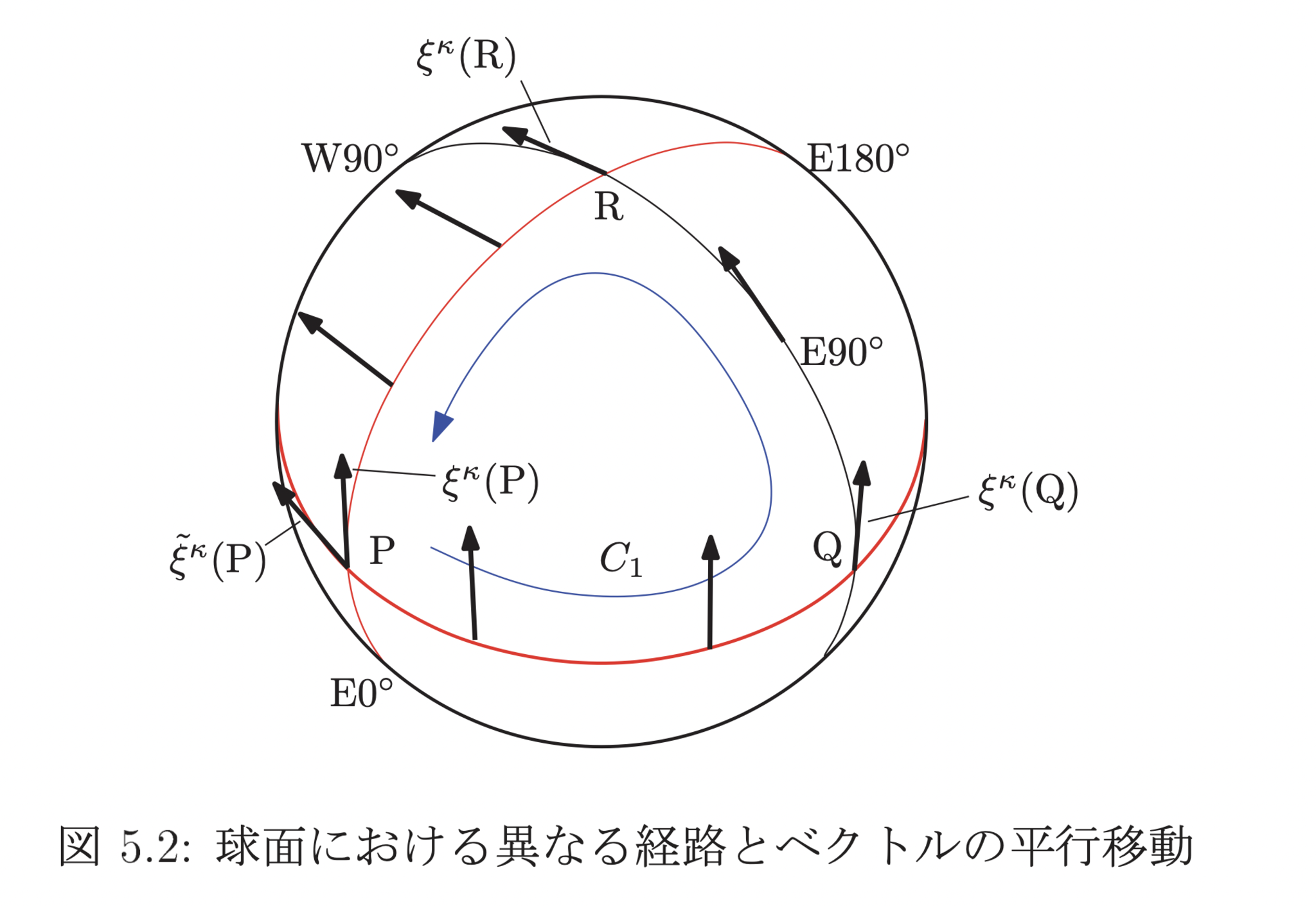 球面における異なる経路とベクトルの平行移動
微小並進移動が演算子$1+h\p$で実現できることを踏まえて、ベクトルの平行移動を成分表示で行ってみる。$x^\nu$方向の微小並進移動は物理流の表記で言えば$v'^\alpha= v^\alpha+h(\p_\nu v^\alpha+\Gamma^\alpha_{~~\beta\nu}v^\beta)$となる。ここまでは共変微分の基本的な話である。では有限距離のベクトルの平行移動はどういう演算子だろう。$v^\bullet,\Gamma^\bullet_{~~\bullet \nu}$の$\bullet$部分を適切にそれぞれ1次元,2次元配列として並べれば行列の線形変換として共変微分の演算を書ける。
$$
\left(
\begin{array}{cc}
~\\
v'^\bullet\\
~
\end{array}
\right)=\begin{eqnarray}
\left(\left(
\begin{array}{cc}
1+h\p_\nu&~&~\\
~&\ddots&~\\
~&~&1+h\p_\nu
\end{array}
\right)+h\left(
\begin{array}{cc}
~&~&~\\
~&\Gamma^\bullet_{~~\bullet \nu}&~\\
~&~&~
\end{array}
\right)\right)
\left(
\begin{array}{cc}
~\\
v^\bullet\\
~
\end{array}
\right)
\end{eqnarray}
$$
さて、スカラー値関数の時同様、区間を等分割して並進移動を繰り返すことで有限距離の並進移動演算子は次のようになる。
$$(v'^\bullet)=e^{a\nabla_\nu}\cdot (v^\bullet)=\exp a[I\p_\nu+(\Gamma^\bullet_{~~\bullet \nu})]~~ (v^\bullet)$$
指数関数の肩に微分演算子と行列が乗った形の複雑な演算子である。具体例を出して実際に計算してみる。
球面座標系$\mathbf r=(\te,\phi)=(x,y,z)=(R\sin\te\cos\phi,R\sin\te\sin\phi,R\cos\te)$においてChristoffel記号は
$$(\Gamma^\bullet_{~~\bullet \te})=\left(
\begin{array}{cc}
\Gamma^\te_{~~\te \te}&\Gamma^\te_{~~\fi \te}\\
\Gamma^\fi_{~~\te \te}&\Gamma^\fi_{~~\fi \te}
\end{array}
\right)=\left(\begin{array}{cc}
0&0\\
0&\cot\te
\end{array}\right)$$
$$(\Gamma^\bullet_{~~\bullet \phi})=\left(
\begin{array}{cc}
\Gamma^\te_{~~\te \fi}&\Gamma^\te_{~~\fi \fi}\\
\Gamma^\fi_{~~\te \fi}&\Gamma^\fi_{~~\fi \fi}
\end{array}
\right)=\left(\begin{array}{cc}
0&-\sin\te\cos\te\\
\cot\te&0
\end{array}\right)$$
となる。ベクトルの基底は$$e_\te=\frac{\p \mathbf r}{\p \te}=(R\cos\te\cos\fi,R\cos\te\sin\fi,-R\sin\te)$$$$e_\fi=\frac{\p \mathbf r}{\p \fi}=(-R\sin\te\sin\fi,R\sin\te\cos\fi,0)$$
$AB=BA$ならば$\exp(A+B)=\exp A\exp B$
$\p_x\cdot f(x)=[\p_x,f(x)]=f'(x)$
heisenberg代数参照
コレを用いて
$$\p_x+\p_x\cdot \log f(x)=\p_x-f(x)^{-1}[f(x),\p_x]=f(x)^{-1}\p_x f(x)$$
随伴作用(共役変換)の準同型性
$$C^{-1}f(AB)C=f((C^{-1}AC)(C^{-1}BC))$$
回転行列の$\exp$
$$
\begin{eqnarray}
\exp\left(
\begin{array}{cc}
0&-\te\\
\te&0
\end{array}
\right)=\left(
\begin{array}{cc}
\cos\te&-\sin\te\\
\sin\te&\cos\te
\end{array}
\right)
\end{eqnarray}
$$
$(v^\bullet)=(v^\te,v^\phi)^T$の$\te$方向の並進移動は
\begin{align}
(v'^\bullet)=&\exp a[I(\p_\te)+(\Gamma^\bullet_{~~\bullet \te})]~~ (v^\bullet)\\
=&\exp a\left[ \left(
\begin{array}{cc}
\p_\te&0\\
0&\p_\te
\end{array}
\right)+\p_\te \cdot \log \left(
\begin{array}{cc}
1&0\\
0&\sin\te
\end{array}
\right)\right]~~ \binom{v^\te}{v^\fi}\\
=&\exp a\left[ \left(
\begin{array}{cc}
1&0\\
0&\sin\te
\end{array}
\right)^{-1}\left(
\begin{array}{cc}
\p_\te&0\\
0&\p_\te
\end{array}
\right)\left(
\begin{array}{cc}
1&0\\
0&\sin\te
\end{array}
\right)\right]~~ \binom{v^\te}{v^\fi}\\
=&\left(
\begin{array}{cc}
1&0\\
0&\sin\te
\end{array}
\right)^{-1}\exp \left(
\begin{array}{cc}
a\p_\te&0\\
0&a\p_\te
\end{array}
\right)\left(
\begin{array}{cc}
1&0\\
0&\sin\te
\end{array}
\right)~~ \binom{v^\te}{v^\fi}\\
=&\left(
\begin{array}{cc}
1&0\\
0&\sin\te
\end{array}
\right)^{-1}\exp \left(
\begin{array}{cc}
a\p_\te&0\\
0&a\p_\te
\end{array}
\right)~~ \binom{v^\te(\te,\fi)}{v^\fi(\te,\fi)\sin\te}\\
=&\left(
\begin{array}{cc}
1&0\\
0&\sin\te
\end{array}
\right)^{-1} \binom{v^\te(\te+a,\fi)}{v^\fi(\te+a,\fi)\sin(\te+a)}\\
=&\binom{v^\te(\te+a,\fi)}{v^\fi(\te+a,\fi)\sin(\te+a)/\sin\te}
\end{align}
となる。計算結果は考える以前に当たり前である。$\te$方向の移動は測地線に沿うので向きが変化せず基底の長さだけが変化し、基底$e_\fi$の長さはその緯度の緯線の長さ(余緯度の正弦)に比例して$\sin\te/\sin(\te+a)$倍され$\fi$成分は反比例する、つまり移動後はその逆比倍されるのである。
$\fi$方向の移動は
\begin{align}
(v'^\bullet)=&\exp a[\mathrm{diag}(\p_\fi)+(\Gamma^\bullet_{~~\bullet \fi})]~~ (v^\bullet)\\
=&\exp a\left[ \left(
\begin{array}{cc}
\p_\fi&0\\
0&\p_\fi
\end{array}
\right)+\left(
\begin{array}{cc}
1&0\\
0&\sin\te
\end{array}
\right)^{-1} \left(
\begin{array}{cc}
0&-\cos\te\\
\cos\te&0
\end{array}
\right) \left(
\begin{array}{cc}
1&0\\
0&\sin\te
\end{array}
\right)\right]~~ \binom{v^\te}{v^\fi}\\
=&\left(
\begin{array}{cc}
1&0\\
0&\sin\te
\end{array}
\right)^{-1}\exp \left(
\begin{array}{cc}
a\p_\fi&0\\
0&a\p_\fi
\end{array}
\right) \exp\left(
\begin{array}{cc}
0&-a\cos\te\\
a\cos\te&0
\end{array}
\right)\left(
\begin{array}{cc}
1&0\\
0&\sin\te
\end{array}
\right)~~ \binom{v^\te}{v^\fi}\\
=&\left(
\begin{array}{cc}
\cos(a\cos\te)&-\sin\te\sin(a\cos\te)\\
{\sin(a\cos\te)}/{\sin\te}&\cos(a\cos\te)
\end{array}
\right)\binom{v^\te(\te,\fi+a)}{v^\fi(\te,\fi+a)}
\end{align}
という結果になる。回転角$a\cos \te$は$\te=\pi/2$のとき$0$になるが、これは赤道上の移動は測地線(大円)を通ることからも理解できる。
計算の観点的には、ただ$exp(\nabla)$を計算したにもかかわらず二重指数$\cos(a\cos\te)$が現れるのは面白い。
赤道直下の一点で,地面に北向きのベクトル$v_0$を描き、$v_0$を赤道に沿って角度$A$動かしたものを$v_1$として、$v_0,v_1$両方を北極へ向けて平行移動したものをそれぞれ$v_2,v_3$とする。
$$v_0=\binom{1}{0}=\binom{v^\te(\pi/2,0)}{v^\fi(\pi/2,0)}$$
$\sin\epsilon\approx \epsilon$として計算する。
$$v_1(\pi/2,A)=e^{-A\nabla_\fi}\cdot v_0(\pi/2,A)=\binom 10$$
$$v_2(\epsilon,0)=\exp\q{\q{\frac{\pi}2-\epsilon}\nabla_\te}\cdot v_0(\epsilon,0)=\binom{1}{0}$$
$$v_3(\epsilon,A)=\exp\q{\q{\frac{\pi}2-\epsilon}\nabla_\te}\cdot v_1(\epsilon,A)=\binom{1}{0}$$
$$v_3(\epsilon,0)=\left.e^{A\nabla_\fi}\cdot v_3(\te,\fi)\right|_{(\te,\fi)=(\epsilon,0)} =\left(
\begin{array}{cc}
\cos A&-\epsilon \sin A\\
\sin (A) /\epsilon&\cos A
\end{array}
\right)\binom{1}{0}=\binom{\cos A}{\sin (A) /\epsilon}$$
となって確かに長さは変わらず角度が$A$ずれる。
今度は$\R^2$上の極座標表示でベクトルを並進移動することを考える。
$$\mathbf r=\binom xy=\binom{r\cos\te}{r\sin\te}$$
$$e_r=\binom{\cos\te}{\sin\te},~~e_\te=\binom{-r\sin\te}{r\cos\te}$$
$$(\Gamma^\bullet_{~~\bullet r})=\left(
\begin{array}{cc}
0&0\\
0&1/r
\end{array}
\right),~~(\Gamma^\bullet_{~~\bullet \te})=\left(
\begin{array}{cc}
0&-r\\
1/r&0
\end{array}
\right)$$
ベクトル$(v)$の$(u^r,u^\te)$方向の移動は
\begin{align}
(v')=&\exp\q{u^r\nabla_r+u^\te \nabla_\te}\cdot (v)\\
=&\exp\q{(u^r\p_r+u^\te\p_\te)+\left(
\begin{array}{cc}
0&-u^\te r\\
u^\te/r&u^r/r
\end{array}
\right)}\binom{v^r}{v^\te}\\
=&\left(
\begin{array}{cc}
1&0\\
0&r
\end{array}
\right)^{-1}\exp\q{(u^r\p_r+u^\te\p_\te)+\left(
\begin{array}{cc}
0&-u^\te\\
u^\te&0
\end{array}
\right)}\left(
\begin{array}{cc}
1&0\\
0&r
\end{array}
\right)\binom{v^r}{v^\te}\\
=&\left(
\begin{array}{cc}
1&0\\
0&r
\end{array}
\right)^{-1}e^{u^r\p_r}e^{u^\te\p_\te}\left(
\begin{array}{cc}
\cos u^\te&-\sin u^\te\\
\sin u^\te&\cos u^\te
\end{array}
\right)\left(
\begin{array}{cc}
1&0\\
0&r
\end{array}
\right)\binom{v^r}{v^\te}\\
=&\left(
\begin{array}{cc}
v^r(r+u^r,\te+u^\te)\cos u^\te-rv^\te(r+u^r,\te+u^\te)\sin u^\te\\
\frac 1r v^r(r+u^r,\te+u^\te)\sin u^\te+\frac{r+u^r}{r}v^\te(r+u^r,\te+u^\te)\cos u^\te
\end{array}
\right)
\end{align}
となる。
演算子的にRicciの公式を理解することも可能である。
Riemann曲率テンソル
$$R^i_{~jkl}=\frac{\p \Gamma^i_{~lj}}{\p u^k}-\frac{\p \Gamma^i_{~kj}}{\p u^l}+\Gamma^i_{~kn}\Gamma^n_{~lj}-\Gamma^i_{~ln}\Gamma^n_{~kj}$$に対して
$$\nabla_k\nabla_l v^i-\nabla_l\nabla_k v^i=R^i_{~jkl}v^j$$
が成立する。
これは偏微分演算子同士は可換なので
\begin{align}
&[\nabla_k,\nabla_l](v^\bullet)\\
=&\q{[\p_k,\p_l]+[\p_k,(\Gamma^\bullet_{~~\bullet l})]-[\p_l,(\Gamma^\bullet_{~~\bullet k})]+[(\Gamma^\bullet_{~~\bullet k}),(\Gamma^\bullet_{~~\bullet l})]}(v^\bullet)\\
=&\q{\frac{\p(\Gamma^\bullet_{~~\bullet l})}{\p u^k}-\frac{\p(\Gamma^\bullet_{~~\bullet k})}{\p u^l}+[(\Gamma^\bullet_{~~\bullet k}),(\Gamma^\bullet_{~~\bullet l})]}(v^\bullet)\\
=&(R^\bullet_{~~\bullet kl})(v^\bullet)
\end{align}
という風に証明できる。ただし$(R^\bullet_{~~\bullet kl})$はRiemann曲率テンソルの成分をうまく2次元配列(行列)でならべたものである。微小並進で$u^\mu,u^\nu$方向の微小四角形の上をベクトルがシフトする状況を考えたとき指数関数を2次の項まで展開することで
\begin{align}
&\exp\q{du^\mu\nabla_\mu}\exp\q{du^\nu\nabla_\nu}\exp\q{-du^\mu\nabla_\mu}\exp\q{-du^\nu\nabla_\nu}(v^\bullet)\\
=&(v^\bullet)+du^\mu du^\nu [\nabla_\mu,\nabla_\nu](v^\bullet)\\
=&(v^\bullet)+du^\mu du^\nu(R^\bullet_{~~\bullet \mu\nu})(v^\bullet)
\end{align}
となって自然にRiemann曲率テンソルが現れる。空間の局所的な歪みの大きさを、面積に対する周回によるズレの大きさで計ることができることを意味している。