tikz-3dplotを用いない立体描画
概要
TikZで平面図形を描くのは比較的シンプルなコマンドで実現でき、日本語での解説も豊富にあります。本記事で使用するコマンドに関しては参考文献TikZ-1,TikZ-2,TikZ-3に載っています。これに対して立体図形は、tikz-3dplotなどの派生パッケージで描けるもののコマンドが複雑であり、日本語での解説も多くありません。ということで、平面図形用のコマンドだけで立体図形を描くことにしました。なお、以下では見栄えの都合上、座標を横ヴェクトルで表示します。
目標
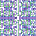
ここでは以下のような図の描画を目的とします。
 描画例
描画例
ソースコードはこちら:
      \newcommand\project[3]{{(2*(#1)+(#2))/sqrt(5)},{(-(#1)+2*(#2)+5*(#3))/sqrt(30)}}
\newcommand\polarproj[3]{\project{(#1)*cos(#2)*cos(#3)}{(#1)*sin(#2)*cos(#3)}{(#1)*sin(#3)}}
% 九九九の表
\begin{tikzpicture}[scale=0.6]
\foreach \x in {1, 2, ..., 9}{
    \foreach \y in {9, 8, ..., 1}{
        \foreach \z in {1, 2, ..., 9}{
            \draw[fill=white, thick](\project\x\y\z)circle(0.5)node{\pgfmathparse{int(\x*\y*\z)}$\pgfmathresult$};
        }
    }
}
\end{tikzpicture}\qquad
% レムニスケートの半分の回転体
% r^2=-cos2φ, (x,y,z)=(rcosθcosφ,rsinθcosφ,rsinφ), 0<z
\begin{tikzpicture}[scale=8]
% 経線?
\newcommand\varphiborder{atan(2*sin(\longitude)-cos(\longitude))/3}
\foreach \longitude in {15, 30, 45}
\draw[domain=\varphiborder+60:\varphiborder+120, variable=\latitude, samples=100]plot(\polarproj{sqrt(-cos(2*\latitude))}\longitude\latitude);
\foreach \longitude in {60, 75, 90, ..., 180}
\draw[domain=\varphiborder+60:135, variable=\latitude, samples=100]plot(\polarproj{sqrt(-cos(2*\latitude))}\longitude\latitude);
% 緯線?
\newcommand\thetaborder{acos(-tan(3*\latitude)/sqrt(5))}
\foreach \latitude in {46, 49, ..., 79}
\draw[domain=360-\thetaborder-atan(2):360+\thetaborder-atan(2), variable=\longitude, samples=100]plot(\polarproj{sqrt(-cos(2*\latitude))}\longitude\latitude);
\foreach \latitude in {82, 85, 88}
\draw[domain=0:360, variable=\longitude, samples=100]plot(\polarproj{sqrt(-cos(2*\latitude))}\longitude\latitude);
% 輪郭線
\newcommand\latitude{(\varphiborder+60)}
\draw[thick, domain=0:360-acos(1/sqrt(5))-atan(2), variable=\longitude, samples=100]plot(\polarproj{sqrt(-cos(2*\latitude))}\longitude\latitude);
\end{tikzpicture}
射影
この図は、立体をある方向から見たときの様子になっています。もう少し数学的な言葉で言えば、ある平面への射影です。$2$点$\mathrm A,\mathrm B$が重なって見える方向から見ているとすれば、射影先の平面は直線$\mathrm{AB}$に直交する平面です。例として、点$\mathrm A$の座標を$(0,2,0)$, 点$\mathrm B$の座標を$(1,0,1)$とした場合を考えると、直線$\mathrm{AB}$の方向ヴェクトルは$(1,-2,1)$なので、原点を通って直線$\mathrm{AB}$に直交する平面は$\langle(1,-2,1)\rangle$の直交補空間になります。
\begin{align*}
\langle(1,-2,1)\rangle^\perp&=\{\boldsymbol x\in\mathbb R^3\mid \boldsymbol x\cdot(1,-2,1)=0\}\\
&=\{(x,y,z)\in\mathbb R^3\mid x-2y+z=0\}
\end{align*}
点$(x,y,z)$をこの平面に射影して得られる点、即ち点$(x,y,z)$から$\langle(1,-2,1)\rangle^\perp$へ下ろした垂線の足の座標$(x',y',z')$を求めましょう。実数$t$を用いて
$$(x',y',z')=(x,y,z)+t(1,-2,1)=(x+t,y-2t,z+t)$$
と表すことができ、$x'-2y'+z'=0$から$t=-\dfrac{x-2y+z}6$が分かるので、
$$(x',y',z')=\frac16\left(5x+2y-z,2x+2y+2z,-x+2y+5z\right)$$
です。これで三次元空間上の点を平面に落とし込むことができました。次ににこれを$\mathbb R^2$上の点に変換します。そのために$\langle(1,-2,1)\rangle^\perp$の正規直交基底を構成しましょう。まず適当に$(2,1,0),(0,1,2)\in\langle(1,-2,1)\rangle^\perp$をとってくるとこれは基底になっています。これにGram-Schmidtの正規直交化法を使うと
\begin{align*}
\boldsymbol e_1&=\frac1{\|(2,1,0)\|}(2,1,0)=\frac1{\sqrt5}(2,1,0)\\
\boldsymbol e_2'&=(0,1,2)-(\boldsymbol e_1\cdot(0,1,2))\boldsymbol e_1=\left(-\frac25,\frac45,2\right)\\
\boldsymbol e_2&=\frac1{\|\boldsymbol e_2\|}\boldsymbol e_2=\frac1{\sqrt{30}}(-1,2,5)
\end{align*}
となるので、$\langle(1,-2,1)\rangle^\perp=\left\langle\boldsymbol e_1,\boldsymbol e_2\right\rangle$が正規直交基底として得られます。この基底を使って$(x',y',z')=X\boldsymbol e_1+Y\boldsymbol e_2$と表すとき、$z$座標を考えることにより$Y=\dfrac{\sqrt{30}}5z'$が、$y$座標を考えることにより$X=\sqrt5\left(y'-\dfrac25z'\right)$が分かります。以上をまとめると、
\begin{align*}
\begin{pmatrix}X\\Y\end{pmatrix}&=\begin{pmatrix}0&\sqrt5&-2/\sqrt5\\0&0&\sqrt{30}/5\end{pmatrix}\begin{pmatrix}x'\\y'\\z'\end{pmatrix}\\
&=\begin{pmatrix}0&\sqrt5&-2/\sqrt5\\0&0&\sqrt{30}/5\end{pmatrix}\cdot\frac16\begin{pmatrix}5&2&-1\\2&2&2\\-1&2&5\end{pmatrix}\begin{pmatrix}x\\y\\z\end{pmatrix}\\
&=\begin{pmatrix}2/\sqrt5&1/\sqrt5&0\\-1/\sqrt{30}&2/\sqrt{30}&5/\sqrt{30}\end{pmatrix}\begin{pmatrix}x\\y\\z\end{pmatrix}
\end{align*}
この線型写像による像を描画します。自分で行列計算をして結果をソースコードに書き入れるとごちゃごちゃするので、
      % (\project{x}{y}{z}) -> ({X},{Y})
\newcommand\project[3]{{(2*(#1)+(#2))/sqrt(5)},{(-(#1)+2*(#2)+5*(#3))/sqrt(30)}}
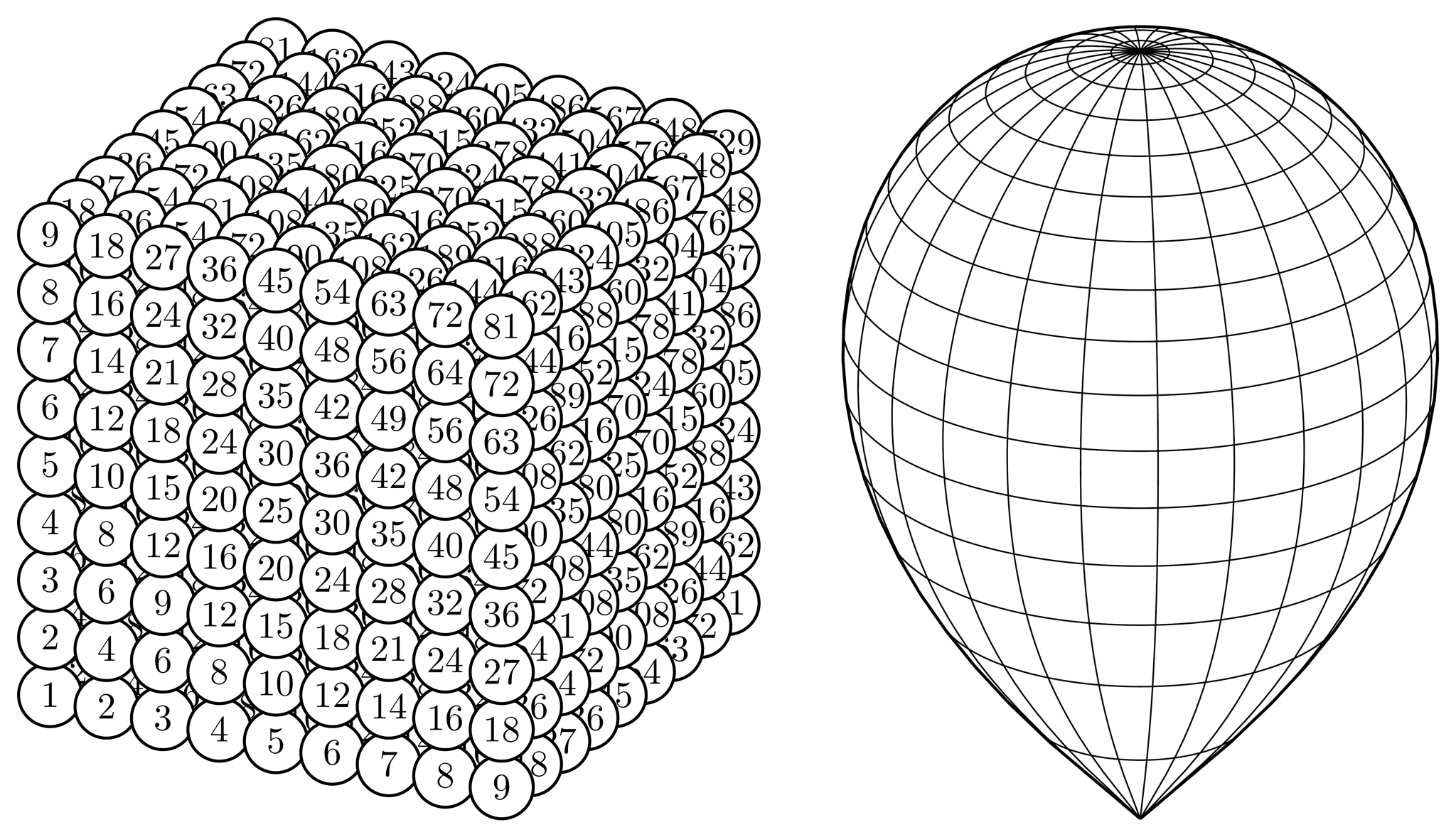
のようにコマンドを定義しておきます。例えば立方体の場合、$(0,0,0)$や$(1,0,1)$などを結べばよいので、
      % 立方体の描画
\newcommand\project[3]{{(2*(#1)+(#2))/sqrt(5)},{(-(#1)+2*(#2)+5*(#3))/sqrt(30)}}
\begin{tikzpicture}
\draw(\project000)--(\project100)--(\project110)--(\project010)--cycle;
\draw(\project001)--(\project101)--(\project111)--(\project011)--cycle;
\draw(\project000)--(\project001);
\draw(\project100)--(\project101);
\draw(\project110)--(\project111);
\draw(\project010)--(\project011);
\end{tikzpicture}
とすればよいです。
 立方体
立方体
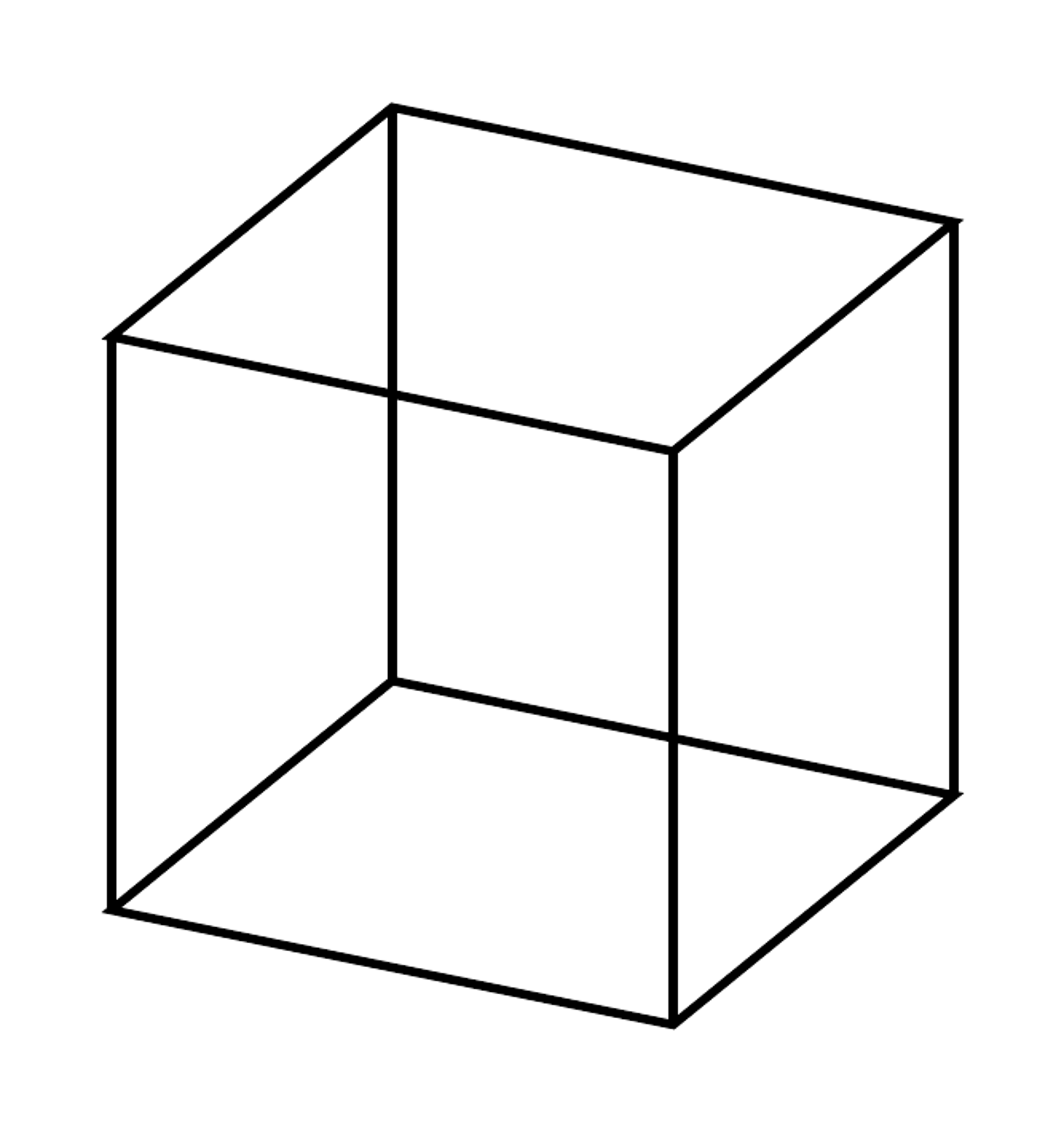
余談ですが、何故かこの図だと奥行きが小さいように見える気がします。透視図法を使えば良いのかもしれませんが…。$(0,10,0)$と$(1,0,1)$が重なるような目線で射影するとさらに薄くなります。単位球面は
$$(x,y,z)=(\cos\theta\cos\varphi,\sin\theta\cos\varphi,\sin\varphi)$$
とパラメータ表示できるので、
      % 球面の描画
\newcommand\project[3]{{(2*(#1)+(#2))/sqrt(5)},{(-(#1)+2*(#2)+5*(#3))/sqrt(30)}}
\begin{tikzpicture}
% 輪郭線
\draw(0,0)circle(1);
% longitude=θ, latitude=φ
% 経線
\foreach \longitude in {15, 30, ..., 180}
\draw[very thin, domain=0:360, variable=\latitude, samples=100]plot(\project{cos(\longitude)*cos(\latitude)}{sin(\longitude)*cos(\latitude)}{sin(\latitude)});
% 緯線
\foreach \latitude in {-75, -60, ..., 75}
\draw[very thin, domain=0:360, variable=\longitude, samples=100]plot(\project{cos(\longitude)*cos(\latitude)}{sin(\longitude)*cos(\latitude)}{sin(\latitude)});
\end{tikzpicture}
とできます。なお、簡便化のため球面座標でプロットするコマンドも作っておきます。
      % 球面の描画 (球面座標系)
\newcommand\project[3]{{(2*(#1)+(#2))/sqrt(5)},{(-(#1)+2*(#2)+5*(#3))/sqrt(30)}}
% (\polarproj{r}{θ}{φ}) -> (\project{rcosθcosφ}{rsinθcosφ}{rsinφ})
\newcommand\polarproj[3]{\project{(#1)*cos(#2)*cos(#3)}{(#1)*sin(#2)*cos(#3)}{(#1)*sin(#3)}}
\begin{tikzpicture}
% 輪郭線
\draw(0,0)circle(1);
% longitude=θ, latitude=φ
% 経線
\foreach \longitude in {15, 30, ..., 180}
\draw[very thin, domain=0:360, variable=\latitude, samples=100]plot(\polarproj1\longitude\latitude);
% 緯線
\foreach \latitude in {-75, -60, ..., 75}
\draw[very thin, domain=0:360, variable=\longitude, samples=100]plot(\polarproj1\longitude\latitude);
\end{tikzpicture}
 単位球
単位球
輪郭
$$(x,y,z)=(\cos\theta(3+\cos\varphi),\sin\theta(3+\cos\varphi),\sin\varphi)$$
でパラメータ表示される二次元トーラスを前節の方法でプロットすると、以下のようになります。
      % トーラスの描画1
\newcommand\project[3]{{(2*(#1)+(#2))/sqrt(5)},{(-(#1)+2*(#2)+5*(#3))/sqrt(30)}}
\begin{tikzpicture}
% longitude=θ, latitude=φ
% 経線?
\foreach \longitude in {10, 20, ..., 360}
\draw[domain=0:360, variable=\latitude, samples=100]plot(\project{cos(\longitude)*(3+cos(\latitude))}{sin(\longitude)*(3+cos(\latitude))}{sin(\latitude)});
% 緯線?
\foreach \latitude in {30, 60, ..., 360}
\draw[domain=0:360, variable=\longitude, samples=100]plot(\project{cos(\longitude)*(3+cos(\latitude))}{sin(\longitude)*(3+cos(\latitude))}{sin(\latitude)});
\end{tikzpicture}
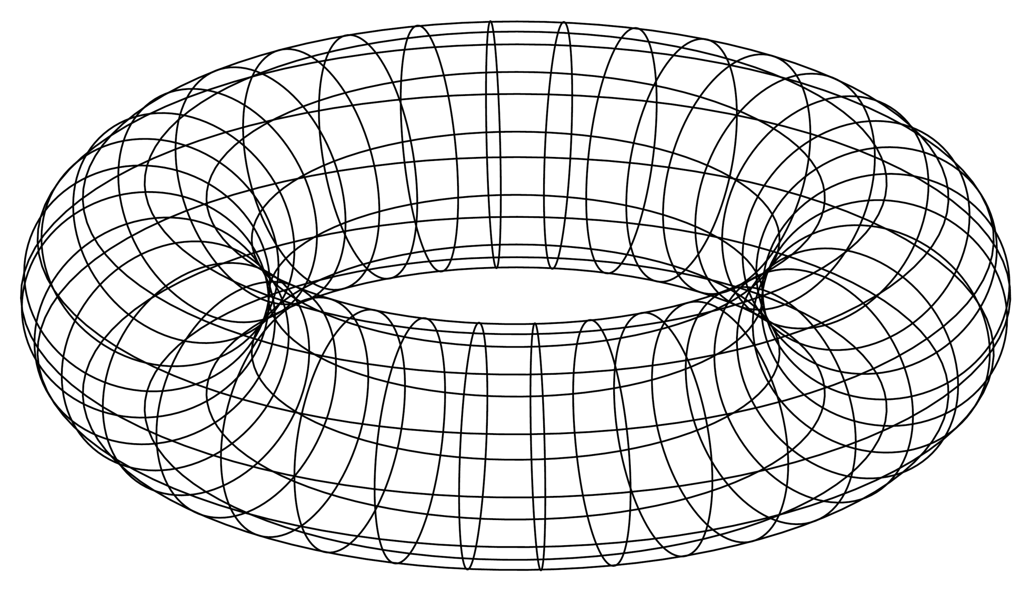 二次元トーラス (美しくない)
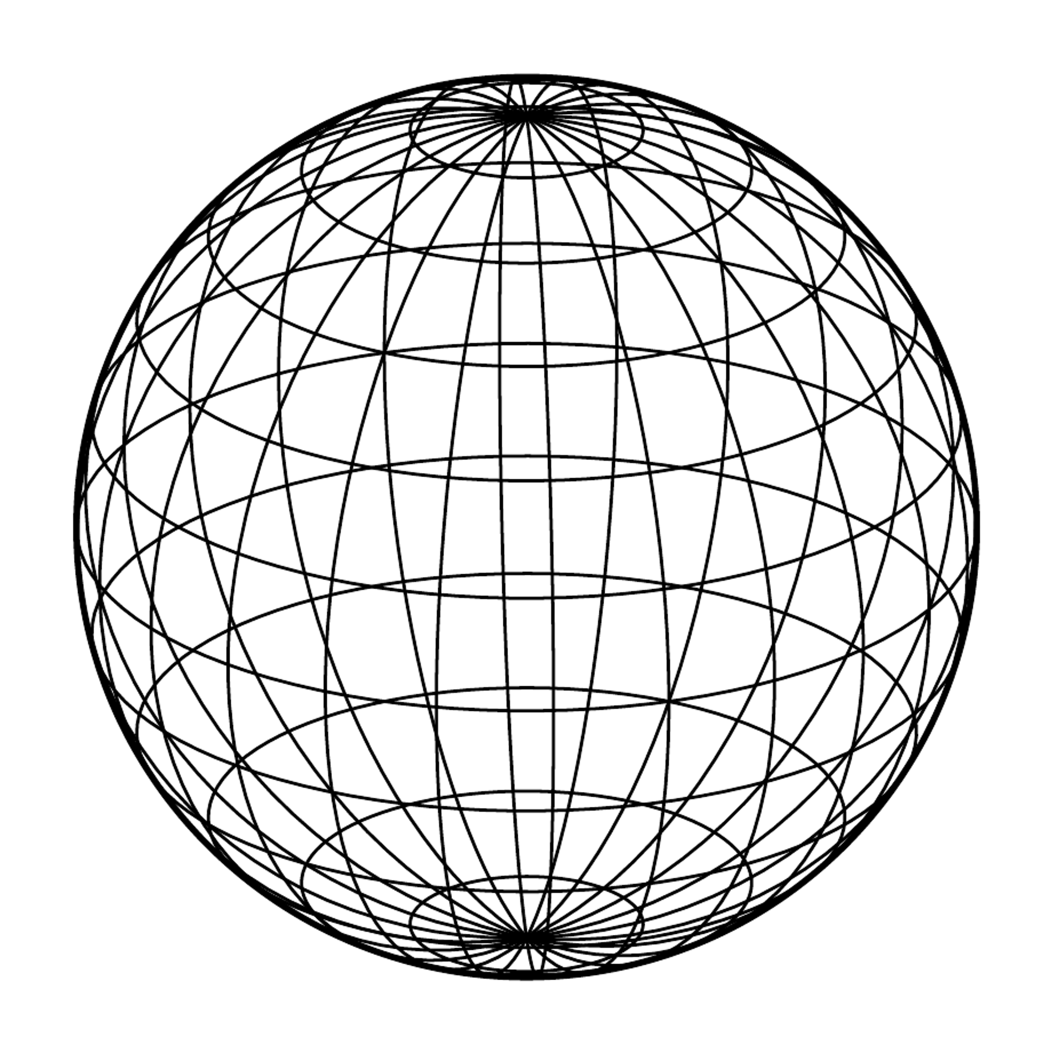
これは美しくありません。本来見えないはずの裏側の線が見えていることが主原因だと考え、見える部分だけを表示するとこうなります(ついでに輪郭線を書き加えておきました)。
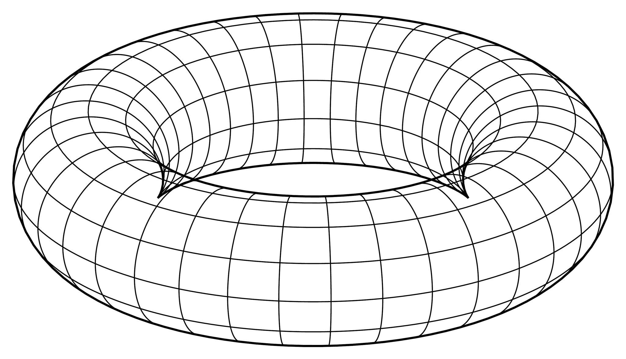 二次元トーラス (美しい)
この図の描画方法を考えましょう。$\theta$を固定して$\varphi$を動かしたり$\varphi$を固定して$\theta$を動かしたりして線を描くわけですが、線が立体の手前側にあるか奥側にあるかの境目は、図における立体の輪郭線に相当します。よって、輪郭の位置を把握すれば表裏を判断できることになります。
$$ f:\mathbb R^2\to\mathbb R^3,(\theta,\varphi)\mapsto(\cos\theta(3+\cos\varphi),\sin\theta(3+\cos\varphi),\sin\varphi)$$
とおくと、点$f(\theta_0,\varphi_0)$におけるトーラスの接平面は
$$\langle f_\theta(\theta_0,\varphi_0),f_\varphi(\theta_0,\varphi_0)\rangle$$
に平行です(証明は省きますが、この部分空間の次元は常に$2$です)。$f(\theta_0,\varphi_0)$を平面に射影した像が輪郭に含まれるのは視線の方向を表す$(1,-2,1)$が接平面に属するとき、即ち
$$\dim\langle f_\theta(\theta_0,\varphi_0),f_\varphi(\theta_0,\varphi_0),(1,-2,1)\rangle<3$$
となる場合なので、3本のヴェクトルから作られる行列式が$0$になる条件を考えればよいことになります。
\begin{align*}
f_\theta(\theta_0,\varphi_0)&=(-\sin\theta(3+\cos\varphi),\cos\theta(3+\cos\varphi),0)\\
f_\varphi(\theta_0,\varphi_0)&=(-\cos\theta\sin\varphi,-\sin\theta\sin\varphi,\cos\varphi)\\
\begin{vmatrix}f_\theta(\theta_0,\varphi_0)\\f_\varphi(\theta_0,\varphi_0)\\(1,-2,1)\end{vmatrix}&=\begin{vmatrix}-\sin\theta(3+\cos\varphi)&\cos\theta(3+\cos\varphi)&0\\-\cos\theta\sin\varphi&-\sin\theta\sin\varphi&\cos\varphi\\1&-2&1\end{vmatrix}\\
&=\sin^2\theta(3+\cos\varphi)\sin\varphi+\cos\theta(3+\cos\varphi)\cos\varphi\\
&\qquad-2\sin\theta(3+\cos\varphi)\cos\varphi+\cos^2\theta(3+\cos\varphi)\sin\varphi\\
&=(3+\cos\varphi)(\sin\varphi-(2\sin\theta-\cos\theta)\cos\varphi)
\end{align*}
$3+\cos\varphi$は常に正ですから、この行列式が$0$になるのは$\sin\varphi=(2\sin\theta-\cos\theta)\cos\varphi$のときです。これを$\theta$と$\varphi$についてそれぞれ解くと、
\begin{align*}
\tan\varphi&=2\sin\theta-\cos\theta=-\sqrt5\cos(\theta+\tan^{-1}2)\\
\theta&=\cos^{-1}\left(-\frac1{\sqrt5}\tan\varphi\right)-\tan^{-1}2\\
\varphi&=\tan^{-1}(2\sin\theta-\cos\theta)
\end{align*}
が解の1つとして求まります。これを基にして曲線の描画範囲を決定します。ここからは厳密に議論するとややこしくなりそうなので、図を見て考えます。まずは$\theta$を固定した場合についてです。$\tan^{-1}$の主値を$(-90^\circ,90^\circ)$でとると(TikZのatanはこの主値の取り方)、
\begin{align*}
\varphi_1&=\tan^{-1}(2\sin\theta-\cos\theta)\\
\varphi_2&=\tan^{-1}(2\sin\theta-\cos\theta)+180^\circ
\end{align*}
$\varphi_1\leqq\varphi\leqq\varphi_2$の範囲を描画することで手前側の曲線になります。次に$\varphi$を固定した場合についてですが、こちらは条件分岐が複雑です。そもそも$\sqrt5<|\tan\varphi|$の場合は$\tan\varphi=2\sin\theta-\cos\theta$の解が存在しません。その中でも図の上側の領域($0<\sin\varphi$)では常にトーラスの手前側に曲線があり、図の下側の領域($\sin\varphi<0$)では常にトーラスの奥側に曲線があります。また、$|\tan\varphi|\leqq\sqrt5$の場合に$\cos^{-1}$の主値を$[0^\circ,180^\circ]$でとって(TikZのacosはこの主値の取り方)
\begin{align*}
\theta_1&=-\cos^{-1}\left(-\frac1{\sqrt5}\tan\varphi\right)-\tan^{-1}2\\
\theta_2&=\cos^{-1}\left(-\frac1{\sqrt5}\tan\varphi\right)-\tan^{-1}2
\end{align*}
と定めるとします。このとき回転軸から見て外側の領域($0<\cos\varphi$)では$\theta_1\leqq\theta\leqq\theta_2$の範囲が手前側になり、回転軸から見て内側の領域($\cos\varphi<0$)では$\theta_2\leqq\theta\leqq\theta_1+360^\circ$の範囲が手前側になります。$\tan^{-1}\sqrt5$は約$65.9^\circ$なので、上の議論から描画範囲は概ね
- $-65.9^\circ<\varphi<65.9^\circ$の場合$\theta_1\leqq\theta\leqq\theta_2$
- $65.9^\circ\leqq\varphi\leqq114.1^\circ$の場合$0^\circ\leqq\theta\leqq360^\circ$
- $114.1^\circ<\varphi<245.9^\circ$の場合$\theta_2\leqq\theta\leqq\theta_1+360^\circ$
とすればよいことが分かります。ということで、先程の図は以下のようにして描けます。
      % トーラスの描画2
\newcommand\project[3]{{(2*(#1)+(#2))/sqrt(5)},{(-(#1)+2*(#2)+5*(#3))/sqrt(30)}}
\begin{tikzpicture}
% longitude=θ, latitude=φ
% 経線?
\newcommand\varphione{atan(2*sin(\longitude)-cos(\longitude))}
\newcommand\varphitwo{\varphione+180}
\foreach \longitude in {10, 20, ..., 360}
\draw[domain=\varphione:\varphitwo, variable=\latitude, samples=100]plot(\project{cos(\longitude)*(3+cos(\latitude))}{sin(\longitude)*(3+cos(\latitude))}{sin(\latitude)});
% 緯線?
\newcommand\thetaone{-acos(-tan(\latitude)/sqrt(5))-atan(2)}
\newcommand\thetatwo{acos(-tan(\latitude)/sqrt(5))-atan(2)}
\foreach \latitude in {-60, -30, ..., 60}
\draw[domain=\thetaone:\thetatwo, variable=\longitude, samples=100]plot(\project{cos(\longitude)*(3+cos(\latitude))}{sin(\longitude)*(3+cos(\latitude))}{sin(\latitude)});
\foreach \latitude in {90}
\draw[domain=0:360, variable=\longitude, samples=100]plot(\project{cos(\longitude)*(3+cos(\latitude))}{sin(\longitude)*(3+cos(\latitude))}{sin(\latitude)});
\foreach \latitude in {120, 150, ..., 240}
\draw[domain=\thetatwo:\thetaone+360, variable=\longitude, samples=100]plot(\project{cos(\longitude)*(3+cos(\latitude))}{sin(\longitude)*(3+cos(\latitude))}{sin(\latitude)});
% 輪郭線
\foreach \latitude in {\varphione, \varphitwo}
\draw[thick, domain=0:360, variable=\longitude, samples=100]plot(\project{cos(\longitude)*(3+cos(\latitude))}{sin(\longitude)*(3+cos(\latitude))}{sin(\latitude)});
\end{tikzpicture}
実例
理論的な話は前節までで終わりです。ここからは実際に、平面図形用のコマンドだけで色々な空間図形を描画してみます。
立方体の切断
立方体を切断する図を描きます。上で描いた立方体は見えない辺も実線で描きましたが、今回は点線で描きます。
      % 立方体の切断
\newcommand\project[3]{{(2*(#1)+(#2))/sqrt(5)},{(-(#1)+2*(#2)+5*(#3))/sqrt(30)}}
\begin{tikzpicture}
% 3つの立方体
\foreach \shift in {0, 4, 8}{
    \draw[thick, shift={(\shift,0)}](\project002)--(\project022)--(\project222)--(\project220)--(\project200)--(\project000)--cycle--(\project202)--(\project222);
    \draw[thick, shift={(\shift,0)}](\project200)--(\project202);
    \draw[thick, dashed, shift={(\shift,0)}](\project020)--(\project220);
    \draw[thick, dashed, shift={(\shift,0)}](\project000)--(\project020)--(\project022);
}
% 三角形の切断面
\fill[red, opacity=0.3](\project200)--(\project222)--(\project002)--cycle;
% 五角形の切断面
\fill[red, opacity=0.3, shift={(4,0)}](\project200)--(\project22{4/3})--(\project122)--(\project012)--(\project00{4/3})--cycle;
% 六角形の切断面
\fill[red, opacity=0.3, shift={(8,0)}](\project100)--(\project210)--(\project221)--(\project122)--(\project012)--(\project001)--cycle;
\end{tikzpicture}
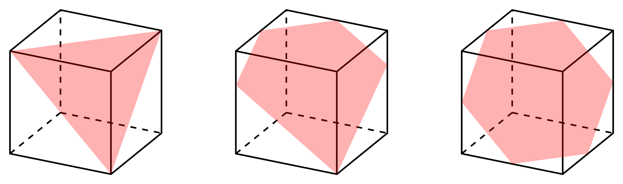 立方体の切断
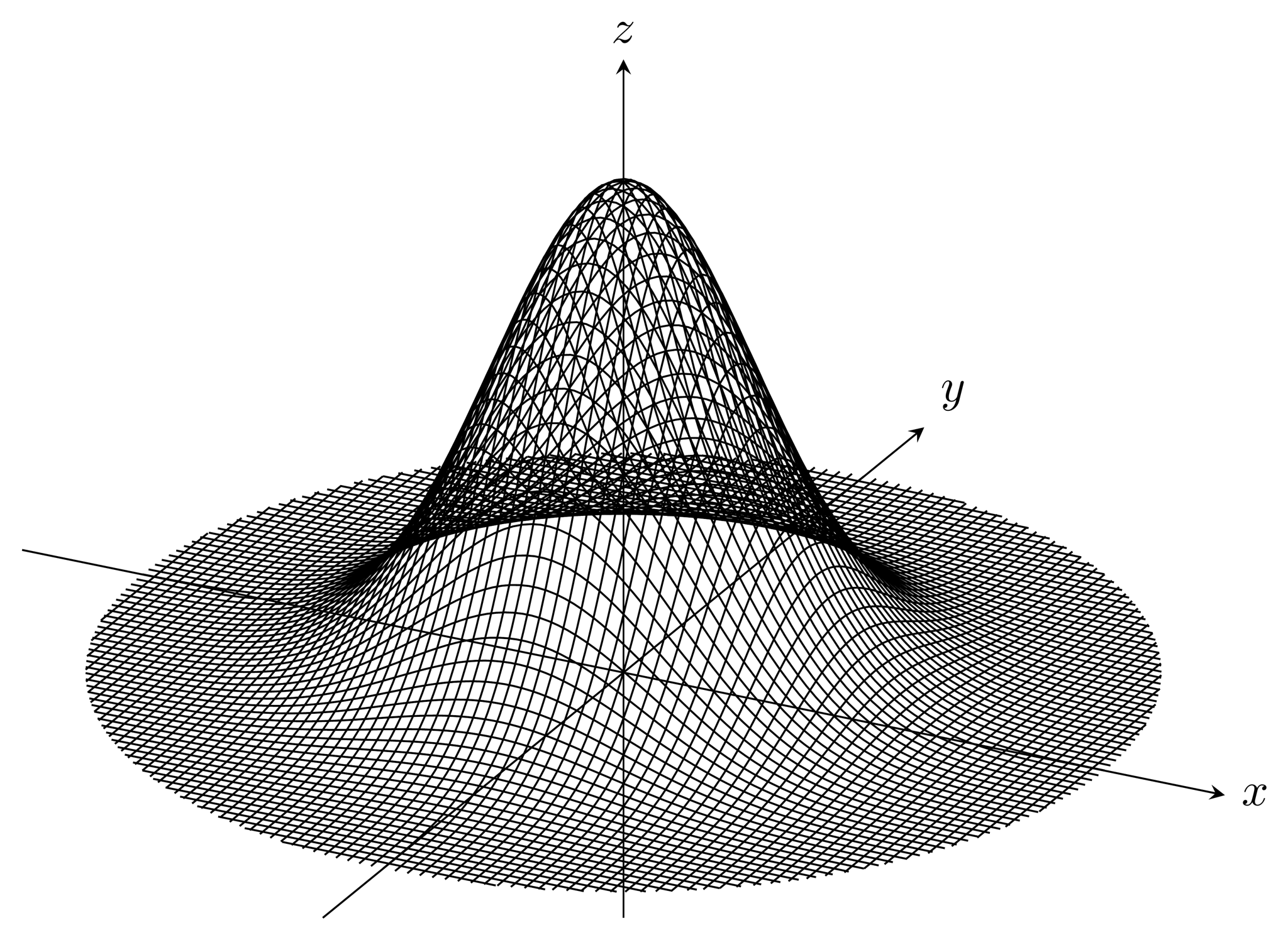
二変数標準正規分布
二変数の標準正規分布の確率密度関数のグラフを描きます。目標はこちら(参考:多変量正規分布)。
 二変数標準正規分布
確率密度函数は$\dfrac1{2\pi}\exp\left(-\dfrac{x^2+y^2}2\right)$で与えられますが、$z$座標が小さくなりすぎないように$16\pi$倍して
$$ f:\mathbb R^2\to\mathbb R^3,(x,y)\mapsto\left(x,y,4\exp\left(-\frac{x^2+y^2}2\right)\right)$$
を描画します。輪郭線を計算しましょう。接平面を生成するヴェクトルは
\begin{align*}
f_x(x,y)=\left(1,0,4x\exp\left(-\frac{x^2+y^2}2\right)\right)\\
f_y(x,y)=\left(0,1,4y\exp\left(-\frac{x^2+y^2}2\right)\right)
\end{align*}
ですから、$\langle f_x(x_0,y_0),f_y(x_0,y_0)\rangle$に$(1,-2,1)$が属する条件は
\begin{align*}
1+4(2y-x)\exp\left(-\frac{x^2+y^2}2\right)=0
\end{align*}
です。この方程式はexplicitに解けません。うまいこと変数変換すれば描画できそうな気がしないでもないですが、思いつかなかったので読者への演習問題とします。とりあえずの完成形はこちら。描画量を多くした結果PCが悲鳴を上げました。
      % 二変数標準正規分布
\newcommand\project[3]{{(2*(#1)+(#2))/sqrt(5)},{(-(#1)+2*(#2)+5*(#3))/sqrt(30)}}
\begin{tikzpicture}
% 座標軸
\draw[-stealth](\project{-5}00)--(\project500)node[right]{$x$};
\draw[-stealth](\project0{-5}0)--(\project050)node[above right]{$y$};
\draw[-stealth](\project00{-2})--(\project005)node[above]{$z$};
% 曲面
\foreach \x in {-4, -3.9, ..., 4}
\draw[domain=-sqrt(16-\x*\x):sqrt(16-\x*\x), variable=\y, samples=100]plot(\project\x\y{4*exp(-(\x*\x+\y*\y)/2)});
\foreach \y in {-4, -3.9, ..., 4}
\draw[domain=-sqrt(16-\y*\y):sqrt(16-\y*\y), variable=\x, samples=100]plot(\project\x\y{4*exp(-(\x*\x+\y*\y)/2)});
\end{tikzpicture}
 二変数標準正規分布
電磁波
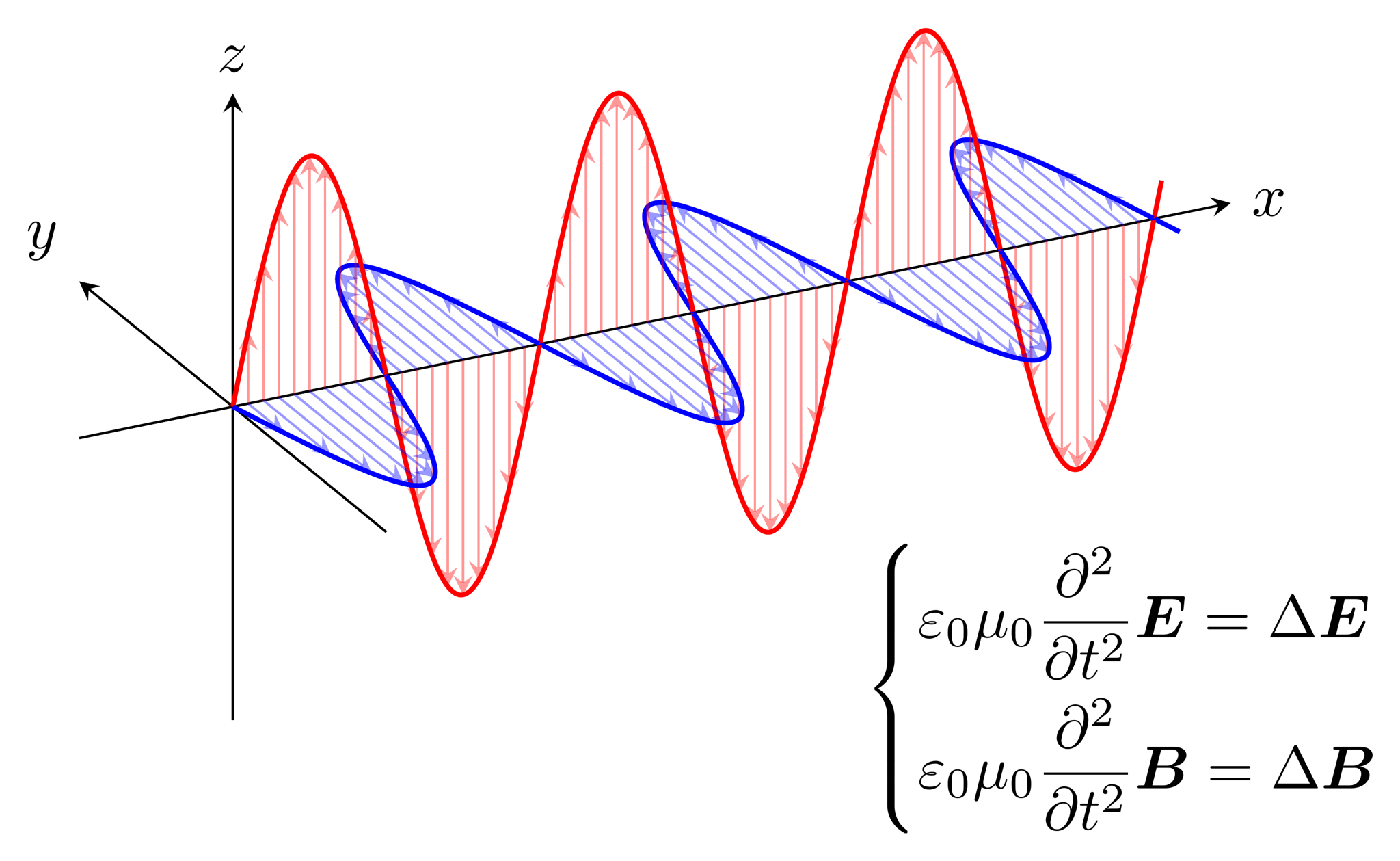
電磁波が伝わる様子を図示します。目標はこちら(参考:電磁波)。
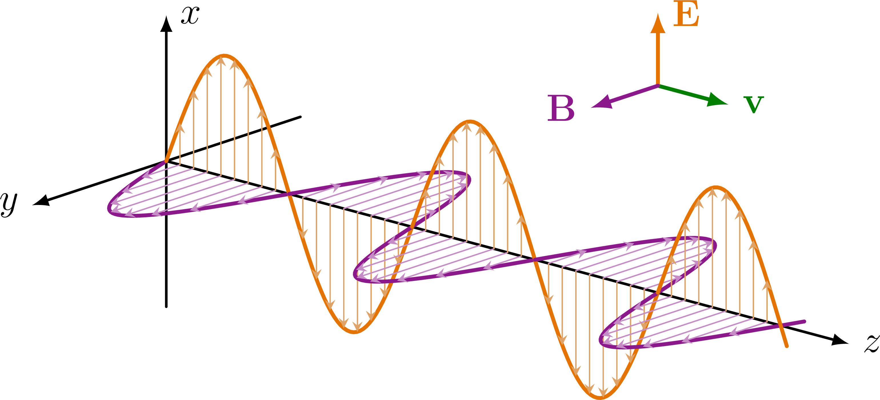 電磁波
電磁波
なんとなく電磁波は右上に向かって進んでほしいので、ここだけ目線の向きを変えます。具体的には、点$(0,2,0)$と点$(-1,0,1)$が重なる方向から見ます。ただし、この座標は参考画像の座標軸でなく、右向きを$x$軸正の方向、奥向きを$y$軸正の方向、上向きを$z$軸正の方向とした座標で考えています。このとき座標変換は
$$\begin{pmatrix}X\\Y\end{pmatrix}=\begin{pmatrix}2/\sqrt5&-1/\sqrt5&0\\1/\sqrt{30}&2/\sqrt{30}&5/\sqrt{30}\end{pmatrix}\begin{pmatrix}x\\y\\z\end{pmatrix}$$
です。また、電場の波は$z=a\sin bx$ ($y=0$), 磁場の波は$y=-a\sin bx$ ($z=0$)の形で表されます。
      % 電磁波
% ここの射影コマンドは他と異なる
\newcommand\waveproject[3]{{(2*(#1)-(#2))/sqrt(5)},{((#1)+2*(#2)+5*(#3))/sqrt(30)}}
\begin{tikzpicture}
% 座標軸
\draw[-stealth](\waveproject{-1}00)--(\waveproject{6.5}00)node[right]{$x$};
\draw[-stealth](\waveproject0{-2}0)--(\waveproject020)node[above left]{$y$};
\draw[-stealth](\waveproject00{-2})--(\waveproject002)node[above]{$z$};
\draw[red, thick, domain=6:6.05]plot(\waveproject\x0{1.5*sin(180*\x)});
\draw[blue, thick, domain=6:6.05]plot(\waveproject\x{-1.5*sin(180*\x)}0);
\foreach \xshift in {5, 4, 3, ..., 0}{
    % 電場
    \draw[red, thick, domain=\xshift:\xshift+1, samples=100]plot(\waveproject\x0{1.5*sin(180*\x)});
    \foreach \xxshift in {0.1, 0.2, ..., 0.9}
    \draw[red, opacity=0.4, -stealth](\waveproject{\xshift+\xxshift}00)--(\waveproject{\xshift+\xxshift}0{1.5*sin(180*(\xshift+\xxshift))});
    % 磁場
    \draw[blue, thick, domain=\xshift:\xshift+1, samples=100]plot(\waveproject\x{-1.5*sin(180*\x)}0);
    \foreach \xxshift in {0.1, 0.2, ..., 0.9}
    \draw[blue, opacity=0.4, -stealth](\waveproject{\xshift+\xxshift}00)--(\waveproject{\xshift+\xxshift}{-1.5*sin(180*(\xshift+\xxshift))}0);
}
% 電磁場の波動方程式
\draw(\waveproject60{-3})node{$\begin{cases}
\varepsilon_0\mu_0\dfrac{\partial^2}{\partial t^2}\bm E=\Delta\bm E\\[.5zh]
\varepsilon_0\mu_0\dfrac{\partial^2}{\partial t^2}\bm B=\Delta\bm B
\end{cases}$};
\end{tikzpicture}
 電磁波
電磁波
参考文献


この記事を高評価した人
この記事に送られたバッジ
投稿者