複素関数を可視化するMathematicaのコード

Mathematicaはグラフを描いたり、数式を量産したり、数学の概念の可視化に便利なツールです。
wolfram cloud というサイトでアカウントを作れば無料で使えます。製品版は高いですが数学好きなら買って損しません！！！
ここでは私が作った複素関数の可視化ツールの紹介とMathematicaの宣伝をします。
追記：コードを少し直しました。

使い方

まずMathematica のノートブックで以下のコードを入力し Shift + Enter をおします。
このコードで可視化関数DrawComplexの定義がされます。

      DrawComplex[func_, center_, length_, mesh_,
   OptionsPattern[
    {
     Opacity -> 0.5,
     ImageSize -> 500,
     PlotRange -> Automatic,
     Epilog -> {},
     Background -> Black,
     PlotPoints -> 20
     }
    ]
   ] :=
  
  Quiet@Module[{w, l, n, n1, n2, tmp, vl, hl, vcl, hcl, RemoveNaN},
    n1 = mesh[[1]];
    n2 = mesh[[2]];
    w = length[[1]]*0.5;
    l = length[[2]]*0.5;
    n = OptionValue[PlotPoints]*Ceiling[2*l];
    RemoveNaN[points_] := Cases[points, {a_, b_} /; NumericQ[a] && NumericQ[b]];
    vl = Table[
      {
       Opacity@OptionValue[Opacity], Thickness[0.005], RGBColor[0, (a + w)/(2 w ), 1],
       Line@RemoveNaN@
         Table[ReIm@func[a + center[[1]] + (tmp + center[[2]]) I], {tmp, -l, l, (2 l)/n}]
       },{a, -w, w, (2 w)/n1}
      ];
     vcl =
     {
      Opacity@OptionValue[Opacity], Thickness[0.005], RGBColor[0, 1, 0],
      Line@RemoveNaN@
        Table[ReIm@func[center[[1]] + (tmp + center[[2]]) I], {tmp, -l, l, (2 l)/n}]
      };
    hl = Table[
      {
       Opacity@OptionValue[Opacity], Thickness[0.005], RGBColor[1, (a + l)/(2 l ), 1],
       Line@RemoveNaN@
         Table[ReIm@func[tmp + center[[1]] + (a + center[[2]]) I], {tmp, -w, w, (2 w)/n}]
       },{a, -l, l, (2 l)/n2}
      ];
    hcl =
     {
      Opacity@OptionValue[Opacity], Thickness[0.005], RGBColor[1, 1, 0],
      Line@RemoveNaN@
        Table[ReIm@func[tmp + center[[1]] + center[[2]] I], {tmp, -w, w, (2 w)/n}]
      };
    Graphics[
     {
      If[n1 == 0, {}, Append[vl, vcl]],
      If[n2 == 0, {}, Append[hl, hcl]],
      OptionValue[Epilog]
      },
     Background -> OptionValue[Background],
     PlotRange -> OptionValue[PlotRange],
     Axes -> True,
     AxesLabel -> {Re, Im},
     LabelStyle -> {White, Directive[12]},
     ImageSize -> OptionValue[ImageSize],
     AxesStyle -> Table[{Opacity[0.4], White}, {2}],
     PlotRangePadding -> None,
     ImagePadding -> 25,
     AspectRatio -> 1
     ]
    ];
    

つぎに以下のようなコードを入力し Shift + Enter をおします。

      DrawComplex[#^2 &, {0, 0}, {1, 1}, {20, 20}, PlotRange -> 0.5 {{-1, 1}, {-1, 1}}, PlotPoints -> 20]
    

すると以下のような図が描かれます。
$w=z^2 $

関数の説明

この関数は$w=f(z)$という複素関数によって、$z$上の方眼紙がどう変形するかを可視化します。
この関数の入力項目は以下のようになります。

      DrawComplex[func_, center_, length_, mesh_, ...]
    

• func_ : 可視化したい関数を入れます。このとき関数$f(z)$の$z$の代わりに#を使います。そして関数の最後に&をつけます。例えば$f(z)=z^2$という関数を可視化したいならfunc_には#^2&と入力します。
• center_ : $z$上の方眼紙の中心を指定します。例えば原点なら{0,0}とします。
• length_ : 方眼紙の縦横の長さを指定します。例えば縦3,横5なら{3,5}とします。
• mesh_ : 方眼紙の縦横のグリッドの数を指定します。
• ... : この部分にはオプションをいれます。これには以下のようなオプションがあります。
  • Opacity : 線の透明度を指定します。
  • PlotRange : プロット領域を指定します。例えば実軸で {-2,2}、虚軸で {-3,3}の領域を指定したい場合は PlotRange->{{-2,2},{-3,3}}と入力します。
  • PlotPoints : 可視化の細かさを示します。

例

• $w=1/z$

      DrawComplex[1/# &, {0, 0}, {1, 1}, {20, 20}, 
 PlotRange -> 10 {{-1, 1}, {-1, 1}}, PlotPoints -> 100]
    

$w=1/z$

• ゼータ関数

      DrawComplex[Zeta[#] &, {0, 0}, {1, 100}, {5, 0}, 
 PlotRange -> 10 {{-1, 1}, {-1, 1}}, PlotPoints -> 50]
    

$w=\zeta(z) $

応用

この関数をパーツとしていろんな可視化ができます。
-連射

      Grid[
 Transpose@Partition[
   Table[
    With[{l = {2 \[Pi], 2 \[Pi]}, n = {20, 20}, 
      r = {{-\[Pi], \[Pi]}, {-\[Pi], \[Pi]}}, is = 270},
     Labeled[
      DrawComplex[func, {0, 0}, l, n, PlotRange -> r, ImageSize -> is],
      Style[ToString[TraditionalForm@func[z]], White, 18], Top
      ]
     ],
    {func, {Sin, Cos, Tan, Exp, Log, Sinh, Cosh, Tanh}}], 2],
 Background -> Black
 ]
    

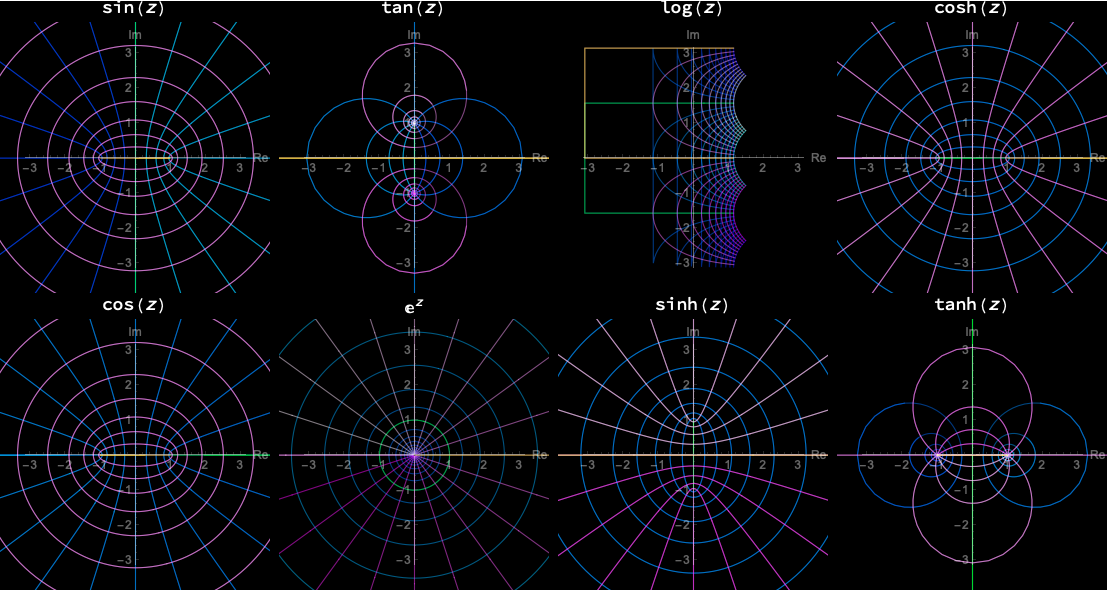いろいろな複素関数
-マウスでドラッグして経路積分ができるコード（Wolfram Cloud 無料版では重すぎる）

      Manipulate[
 DynamicModule[
  {zplane, wplane, iplane, ztraj = {{{0, 0}, {0, 0}}}, 
   wtraj = {{{0, 0}, {0, 0}}}, itraj = {{{0, 0}, {0, 0}}},
   znew, wnew, inew, zold, wold, iold, w, dz, size = 400},
  zplane = 
   DrawComplex[# &, center, length, mesh, PlotRange -> r1, 
    PlotPoints -> 10, ImageSize -> size];
  wplane = 
   DrawComplex[Evaluate[func /. z -> #] &, center, length, mesh, 
    PlotRange -> r2, PlotPoints -> n, ImageSize -> size];
  iplane = 
   DrawComplex[# &, 
    center, (r3[[1, 2]] - r3[[1, 1]]) {1, 1}, {10, 10}, 
    PlotRange -> r3, PlotPoints -> 10, ImageSize -> size];
  EventHandler[
   Dynamic@Grid[
     {
      {
       Show[
        zplane,
        Graphics[
         {
          {White, Line[ztraj]},
          {Red, PointSize[Large], Point[First@First@ztraj]},
          {Blue, PointSize[Large], Point[Last@Last@ztraj]}
          }
         ]
        ]
       ,
       Show[
        wplane,
        Graphics[
         {
          {White, Line[wtraj]},
          {Red, PointSize[Large], Point[First@First@wtraj]},
          {Blue, PointSize[Large], Point[Last@Last@wtraj]}
          }
         ]
        ],
       Show[
        iplane,
        Graphics[
         {
          {White, Line[itraj]},
          {Red, PointSize[Large], Point[First@First@itraj]},
          {Blue, PointSize[Large], Point[Last@Last@itraj]}
          }
         ]
        ]
       },
      {Style["z", Italic], 
       Row[{Style["w", Italic], "(", Style["z", Italic], ")"}], 
       Row[{"\[Integral]", Style["w", Italic], "(", 
         Style["z", Italic], ")", Style["dz", Italic]}]}
      }, BaseStyle -> {14, FontFamily -> "Helvetica"}
     ],
   {
    "MouseDragged" :> (
      znew = MousePosition["Graphics"];
      w = func /. z -> ((zold + znew)/2).{1, I};
      wnew = ReIm[w];
      dz = (znew - zold).{1, I};
      inew = ReIm[w*dz];
      AppendTo[ztraj, {zold, znew}];
      AppendTo[wtraj, {wold, wnew}];
      AppendTo[itraj, {iold, iold + inew}];
      zold = znew;
      wold = wnew;
      iold = iold + inew;
      ),
    "MouseDown" :> (
      zold = MousePosition["Graphics"];
      w = func /. z -> zold.{1, I};
      wold = ReIm[w];
      iold = {0, 0};
      ztraj = {{zold, zold}};
      wtraj = {{wold, wold}};
      itraj = {{iold, iold}};
      )
    }
   ]
  ],
 {{func, z, "Function"}},
 {{center, {0, 0}, "Center"}},
 {{length, {2, 2}, "Length"}},
 {{mesh, {10, 10}, "Mesh"}},
 {{r1, {{-1, 1}, {-1, 1}}, "Z Range"}},
 {{r2, {{-1, 1}, {-1, 1}}, "W Range"}},
 {{r3, 2 \[Pi] {{-1, 1}, {-1, 1}}, "W Range"}},
 {{n, 10, "PlotPoints"}}
 ]
    

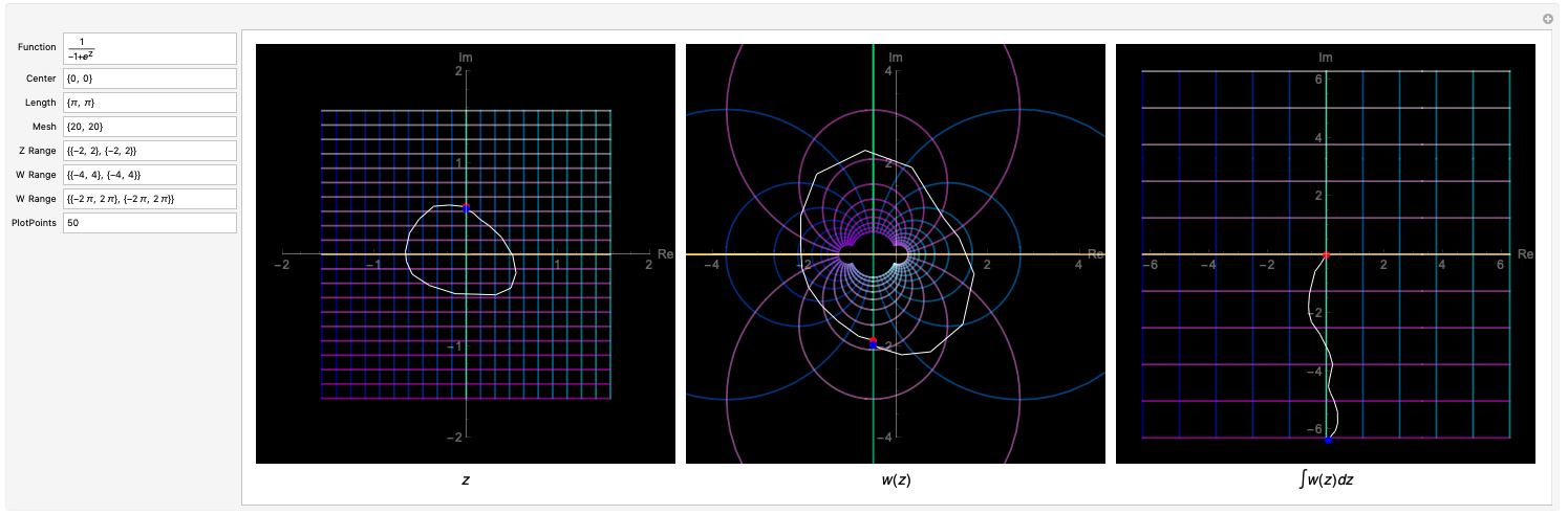経路積分の可視化
以上です。ありがとうございました。